Homework #1 - SQL
Overview
The first homework is to construct a set of SQL queries for analysing a dataset that will be provided to you. For this question you will look into bike sharing data collected from five cities in the Bay Area.
This homework is an opportunity to: (1) learn basic and certain advanced SQL features, and (2) get familiar with using a full-featured DBMS engine, SQLite, that can be useful for you in the future.
This is a single-person project that will be completed individually (i.e., no groups).
- Release Date: Aug 29, 2018
- Due Date: Sep 10, 2018 @ 11:59pm
Specification
The homework contains 10 questions in total and is graded out of 100 points. For each question, you will need to construct a SQL query that fetches the desired data from the SQLite DBMS. It will likely take you approximately 5-7 hours to complete the questions.
We provide the database dump (bike_sharing.tar.gz) on which your queries will be executed. We will also provide a compressed folder (placeholder.zip) containing empty placeholder files
(q1_sample.sql, q2_warmup.sql, ..., q10_riding_in_storm.sql). You will need to fill in the SQL queries in these placeholder files.
You can decompress this folder by running the following command on the terminal:
$ unzip placeholder.zip
After filling in the queries, you can compress the folder by running the following command:
$ zip -j submission.zip placeholder/*.sql
The -j flag lets you flatly compress all the SQL queries in the zip file
without the path.
Instructions
Setting Up SQLite
You will first need to install SQLite on your development machine.
Install SQLite3 on Ubuntu Linux
Install the sqlite3 and libsqlite3-dev packages by running the following command;
$ sudo apt-get install sqlite3 libsqlite3-dev
Install SQLite3 on Mac OS X
On Mac OS Leopard or later, you don't have to! It comes pre-installed. You can upgrade it, if you absolutely need to, with Homebrew.
Load the Database Dump
-
Check if
sqlite3is properly working by following this tutorial. -
Download the database dump file:
$ wget https://15445.courses.cs.cmu.edu/fall2018/files/bike_sharing.tar.gz
- Reconstruct the database from the provided database dump by running the following commands on your shell.
$ tar -zxvf bike_sharing.tar.gz
$ sqlite3 bike_sharing.db < setup.sql
- Check the contents of the database by running the
.tablescommand on thesqlite3terminal. You should see 3 tables, and the output should look like this:
$ sqlite3 bike_sharing.db
SQLite version 3.11.0
Enter ".help" for usage hints.
sqlite> .tables
station  trip     weather
Placeholder Folder
Download the placeholder folder at here:
$ wget https://15445.courses.cs.cmu.edu/fall2018/files/placeholder.zip
$ unzip placeholder.zip
This should contain empty placeholder files
(q1_sample.sql, q2_warmup.sql, ..., q10_riding_in_storm.sql).
Check the schema
Get familiar with the schema (structure) of the tables (what attributes do they contain, what are the primary and foreign keys, etc.). Run the .schema $TABLE_NAME command on the sqlite3 terminal for each table. The output should look like this:
sqlite> .schema station
    CREATE TABLE station(
            station_id smallint not null,
            station_name text,
            lat real,
            long real,
            dock_count smallint,
            city text,
            installation_date date,
            zip_code text,
            PRIMARY KEY (station_id)
    );
sqlite> .schema trip
    CREATE TABLE trip(
            id integer not null,
            duration integer,
            start_time timestamp,
            start_station_name text,
            start_station_id smallint,
            end_time timestamp,
            end_station_name text,
            end_station_id smallint,
            bike_id smallint,
            PRIMARY KEY (id),
            FOREIGN KEY (start_station_id) REFERENCES  station(station_id),
            FOREIGN KEY (end_station_id) REFERENCES  station(station_id)
    );
sqlite> .schema weather
    CREATE TABLE weather(
            date date not null,
            max_temp real,
            mean_temp real,
            min_team real,
            max_visibility_miles real,
            mean_visibility_miles real,
            min_visibility_miles real,
            max_wind_speed_mph real,
            mean_wind_speed_mph real,
            max_gust_speed_mph real,
            cloud_cover real,
            events text,
            wind_dir_degrees real,
            zip_code text not null,
            PRIMARY KEY (date, zip_code)
    );
The following figure illustrates the schema of these tables:
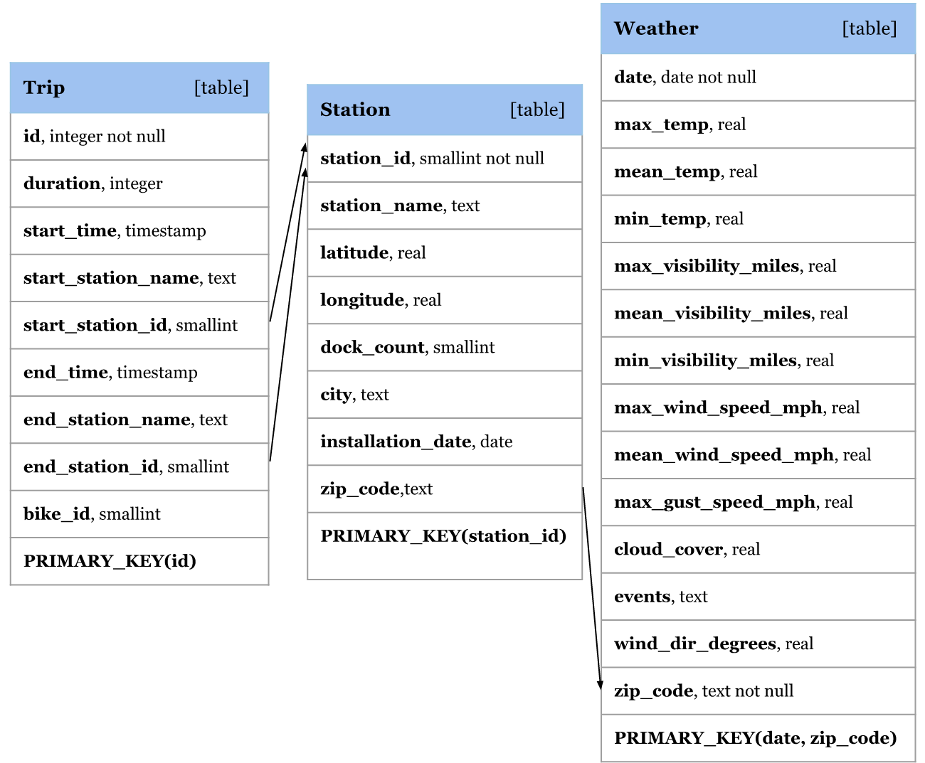
For
example, the tuple in
trip
table
(5088, 183, "2013-08-29 22:08:00", "Market at 4th", 76, "2013-08-29 22:12:00", "Post at Kearney", 47, 309)means that the bike #309 had a trip #5088 from station #76 "Market at 4th" at 2013- 08-29 22:08:00 to station #47 "Post at Kearney" at 2013-08-29 22:12:00.
The tuple in station table
(2, "San Jose Diridon Caltrain Station", 37.3297, -121.902, 27, "San Jose", "2013-08-06", "95113")
means that the station #2 "San Jose Diridon Caltrain Station" in "San Jose" city with latitude as 37.3297, longitude as 121.902, has 27 docks and is installed in 2013-08-06. Its zip code is 95113.
The tuple in weather table
("2013-08-29", 74, 68, 61, 10, 10, 10, 23, 11, 28, 4, "", 286, "94107")
means that in 2013-08-29, the city with zip code "94107" has max temperature 74, mean temperature 68, minimal temperature 61, max visibility miles 10, mean visibility miles 10, maximum wind speed 23 mph, mean wind speed 11 mph, max gust speed 28 mph, cloud cover 4, no special weather events, and wind dir degree 286.
Construct the SQL Queries
Now, it's time to start constructing the SQL queries and put them into the placeholder files.
When calculating the duration of a bike trip, please use trip.start_time and
trip.end_time. Please do NOT use trip.duration, there is inconsistency in
trip.duration in the data we have.
Q1 [0 points] (q1_sample):
Count the number of cities. The purpose of this query is to make sure that the formatting of your output matches exactly the formatting of our auto- grading script.Details: Print the number of cities (eliminating duplicates).
Answer: Here's the correct SQL query and expected output:
sqlite> select count(distinct(city)) from station;
5
You should put this SQL query to the appropriate file (
q1_sample.sql) in the submission directory (placeholder).
Q2 [5 points] (q2_warmup):
Count the number of stations in each city.Details: Print city name and number of stations. Sort by number of stations (increasing), and break ties by city name (increasing).
Q3 [10 points] (q3_popular_city):
Find the percentage of trips in each city. A trip belongs to a city as long as its start station or end station is in the city. For example, if a trip started from station A in city P and ended in station B in city Q, then the trip belongs to both city P and city Q. If P equals to Q, the trip is only counted once.Details: Print city name and ratio between the number of trips that belong to that city against the total number of trips (a decimal between 0-1, round to four decimal places using ROUND()). Sort by ratio (decreasing), and break ties by city name (increasing).
Q4 [15 points] (q4_most_popular_station):
For each city, find the most popular station in that city. "Popular" means that the station has the highest count of visits. As above, either starting a trip or finishing a trip at a station, the trip is counted as one "visit" to that station. The trip is only counted once if the start station and the end station are the same.Details: For each station, print city name, most popular station name and its visit count. Sort by city name, ascending.
Q5 [15 points] (q5_days_most_bike_utilization):
Find the top 10 days that have the highest average bike utilization. For simplicity, we only consider trips that use bikes withid <= 100. The average bike utilization on date D is calculated as the sum of the durations of all the trips that happened on date D divided by the total number of bikes with id <= 100, which is a constant. If a trip overlaps with date D, but starts before date D or ends after date D, then only the interval that overlaps with date D (from 0:00 to 24:00) will be counted when calculating the average bike utilization of date D. And we only calculate the average bike utilization for the date that has been either a start or an end date of a trip. You can assume that no trip has negative time (i.e., for all trips, start time <= end time).
Details: For the dates with the top 10 average duration, print the date and the average bike duration on that date (in seconds, round to four decimal places using the ROUND() function). Sort by the average duration, decreasing.
Please refer to the updated note before Q1 when calculating the
    duration of a trip.
Hint: All timestamps are stored as text after loaded from csv in sqlite. You can use datetime(timestamp string) to get the timestamp out of the string and date(timestamp string) to get the date out of the string. You may also find the funtion strftime() helpful in computing the duration between two timestamps.
Q6 [10 points] (q6_overlapping_trips):
One of the possible data-entry errors is to record a bike as being used in two different trips, at the same time. Thus, we want to spot pairs of overlapping intervals (start time, end time). To keep the output manageable, we ask you to do this check for bikes withid between 100 and 200 (both inclusive). Note: Assume that no trip has negative time, i.e., for all trips, start time <= end time.
Details: For each conflict (a pair of conflict trips), print the bike id, former trip id, former start time, former end time, latter trip id, latter start time, latter end time. Sort by bike id (increasing), break ties with former trip id (increasing) and then latter trip id (increasing).
Hint: (1) Report each conflict pair only once, so that former trip id < latter trip id. (2) We give you the (otherwise tricky) condition for conflicts: start1 < end2 AND end1 > start2
Q7 [10 points] (q7_multi_city_bikes):
Find all the bikes that have been to more than one city. A bike has been to a city as long as the start station or end station in one of its trips is in that city.Details: For each bike that has been to more than one city, print the bike id and the number of cities it has been to. Sort by the number of cities (decreasing), then bike id (increasing).
Q8 [10 points] (q8_bike_popularity_by_weather):
Find what is the average number of trips made per day on each type of weather day. The type of weather on a day is specified by weather.events, such as 'Rain', 'Fog' and so on. For simplicity, we consider all days that does not have a weather event (weather.events = '\N') as a single type of weather. Here a trip belongs to a date only if its start time is on that date. We use the weather at the starting position of that trip as its weather type as well. There are also 'Rain' and 'rain' in weather.events. For simplicity, we consider them as different types of weathers. When counting the total number of days for a weather, we consider a weather happened on a date as long as it happened in at least one region on that date.
Details: Print the name of the weather and the average number of trips made per day on that type of weather (round to four decimal places using ROUND()). Sort by the average number of trips (decreasing), then weather name (increasing).
Q9 [10 points] (q9_temperature_shorter_trips):
A short trip is a trip whose duration is<= 60 seconds. Compute the average temperature that a short trip starts versus the average temperature that a non-short trip starts. We use weather.mean_temp on the date of the start time as the Temperature measurement.
Details: Print the average temperature that a short trip starts and the average temperature
that a non-short trip starts. (on the same row, and both round to four decimal places using
ROUND())
Please refer to the updated note before Q1 when calculating the
    duration of a trip.
Q10 [15 points] (q10_riding_in_storm):
For each zip code that has experienced 'Rain-Thunderstorm' weather, find the station that has the most number of trips in that zip code under the storm weather. For simplicity, we only consider the start time of a trip when deciding the station and the weather for that trip.Details: Print the zip code that has experienced the 'Rain-Thunderstorm' weather, the name of the station that has the most number of trips under the strom weather in that zip code, and the total number of trips that station has under the storm weather. Sort by the zip code (increasing). You do not need to print the zip code that has experienced 'Rain-Thunderstorm' weather but no trip happens on any storm day in that zip code.
Grading Rubric
Each submission will be graded based on whether the SQL queries fetch the expected sets of tuples from the database. Note that your SQL queries will be auto-graded by comparing their outputs (i.e. tuple sets) to the correct outputs. For your queries, the order of the output columns is important; their names are not.
Late Policy
See the late policy in the syllabus.
Submission
We use the Autograder from Gradescope for grading in order to provide you with immediate feedback. After completing the homework, you can submit your compressed folder submission.zip (only one file) to Gradescope:
Important: Use the Gradescope course code announced on Piazza.
We will be comparing the output files using a function similar to diff. You can submit your answers as many times as you like.
Collaboration Policy
- Every student has to work individually on this assignment.
- Students are allowed to discuss high-level details about the project with others.
- Students are not allowed to copy the contents of a white-board after a group meeting with other students.
- Students are not allowed to copy the solutions from another colleague.
WARNING: All of the code for this project must be your own. You may not copy source code from other students or other sources that you find on the web. Plagiarism will not be tolerated. See CMU's Policy on Academic Integrity for additional information.